Introduction to Magnetism and Wave Phenomena
This section covers a range of important physics concepts including magnetism, waves, optics, and nuclear physics. You'll find comprehensive formulas, explanations, and examples for each topic.
Useful Constants
\(\pi = 3.142\) - Mathematical constant representing the ratio of a circle's circumference to its diameter
\(g = 9.80~\mathrm{m/s^2}\) - Acceleration due to gravity at Earth's surface
\(e = 1.6 \times 10^{-19}~\mathrm{C}\) - Elementary charge (charge of an electron or proton)
\(c = 2.998 \times 10^8~\mathrm{m/s}\) - Speed of light in vacuum
\(\mu_0 = 4\pi \times 10^{-7}~\mathrm{Tm/A}\) - Permeability of free space (magnetic constant)
\(m_e = 9.11 \times 10^{-31}~\mathrm{kg}\) - Rest mass of an electron
\(m_p = 1.00728~\mathrm{u}\) - Rest mass of a proton in atomic mass units
\(m_n = 1.00866~\mathrm{u}\) - Rest mass of a neutron in atomic mass units
\(m_{^1\mathrm{H}} = 1.00783~\mathrm{u}\) - Mass of a hydrogen-1 atom in atomic mass units
\(m_{^3\mathrm{H}} = 3.01605~\mathrm{u}\) - Mass of a tritium (hydrogen-3) atom in atomic mass units
Unit Vectors
\(\hat{\imath} \times \hat{\jmath} = \hat{k}\)
\(\hat{\jmath} \times \hat{k} = \hat{\imath}\)
\(\hat{k} \times \hat{\imath} = \hat{\jmath}\)
\(\hat{\jmath} \times \hat{\imath} = -\hat{k}\)
\(\hat{\imath} \times \hat{k} = -\hat{\jmath}\)
\(\hat{k} \times \hat{\jmath} = -\hat{\imath}\)
Vector Cross Products
The cross product (or vector product) is a fundamental operation in vector algebra that produces a vector perpendicular to both input vectors. It's essential for understanding magnetic fields, torque, angular momentum, and many other physics concepts.
Mathematical Definition:
\(\vec{A} \times \vec{B} = \begin{vmatrix} \hat{\imath} & \hat{\jmath} & \hat{k} \\ A_x & A_y & A_z \\ B_x & B_y & B_z \end{vmatrix}\)
\(\vec{A} \times \vec{B} = (A_y B_z - A_z B_y)\hat{\imath} + (A_z B_x - A_x B_z)\hat{\jmath} + (A_x B_y - A_y B_x)\hat{k}\)
Magnitude:
\(|\vec{A} \times \vec{B}| = |\vec{A}||\vec{B}|\sin\theta\)
Where \(\theta\) is the angle between vectors \(\vec{A}\) and \(\vec{B}\)
Key Properties:
- Anti-commutative: \(\vec{A} \times \vec{B} = -\vec{B} \times \vec{A}\)
- Distributive: \(\vec{A} \times (\vec{B} + \vec{C}) = \vec{A} \times \vec{B} + \vec{A} \times \vec{C}\)
- Scalar multiplication: \(k(\vec{A} \times \vec{B}) = (k\vec{A}) \times \vec{B} = \vec{A} \times (k\vec{B})\)
- Parallel vectors: If \(\vec{A} \parallel \vec{B}\), then \(\vec{A} \times \vec{B} = \vec{0}\)
- Self cross product: \(\vec{A} \times \vec{A} = \vec{0}\)
Interactive Vector Cross Product Calculator
Use this calculator to explore vector cross products. Enter the components of two vectors and see the result visualized in real-time.
Vector A
Vector B
Cross Product A × B
Angle between A & B: 90.0°
Physics Applications of Cross Products:
- Magnetic Force: \(\vec{F} = q\vec{v} \times \vec{B}\) - Force on a charge moving in a magnetic field
- Magnetic Field: \(\vec{B} = \frac{\mu_0}{4\pi} \frac{q \vec{v} \times \hat{r}}{r^2}\) - Field created by a moving charge
- Torque: \(\vec{\tau} = \vec{r} \times \vec{F}\) - Rotational effect of a force
- Angular Momentum: \(\vec{L} = \vec{r} \times \vec{p}\) - Rotational momentum
- Angular Velocity: \(\vec{v} = \vec{\omega} \times \vec{r}\) - Velocity in circular motion
Useful Conversions
\(1\,\mathrm{eV} = 1.6 \times 10^{-19}~\mathrm{J}\)
\(1\,\mathrm{u} = 1.661 \times 10^{-27}~\mathrm{Kg} = 931.49\,\mathrm{MeV}/c^2\)
\(1\,\mathrm{Ci} = 3.7 \times 10^{10}~\mathrm{Bq}\)
\(1\,\mathrm{rad} = 0.010~\mathrm{J/Kg}\)
Magnetic Fields
Magnetic Field of a Moving Charge
\(\vec{B} = \frac{\mu_0}{4\pi} \frac{q \vec{v} \times \hat{r}}{r^2} = \frac{\mu_0}{4\pi} \frac{I \vec{\Delta s} \times \hat{r}}{r^2}\)
Where:
- \(\vec{B}\) = magnetic field vector
- \(\mu_0\) = permeability of free space
- \(q\) = electric charge
- \(\vec{v}\) = velocity vector of the charge
- \(\hat{r}\) = unit vector pointing from the charge to the observation point
- \(r\) = distance from the charge to the observation point
- \(I\) = electric current
- \(\vec{\Delta s}\) = displacement vector along the current
This formula, known as the Biot-Savart law, describes the magnetic field created by a moving charge or a current element. The magnetic field at any point in space depends on the charge's velocity, the distance from the charge, and the relative orientation.
Example: A proton with charge \(1.6 \times 10^{-19}\) C moves with a velocity of \(2 \times 10^6\) m/s perpendicular to a line connecting it to an observation point 5 cm away. Calculate the magnetic field at the observation point.
Solution:
Using \(\vec{B} = \frac{\mu_0}{4\pi} \frac{q \vec{v} \times \hat{r}}{r^2}\):
Since the velocity is perpendicular to the line connecting the charge to the observation point, \(|\vec{v} \times \hat{r}| = v\).
\(|\vec{B}| = \frac{4\pi \times 10^{-7} \text{ Tm/A}}{4\pi} \frac{1.6 \times 10^{-19} \text{ C} \times 2 \times 10^6 \text{ m/s}}{(0.05 \text{ m})^2}\)
\(|\vec{B}| = 10^{-7} \times \frac{3.2 \times 10^{-13}}{2.5 \times 10^{-3}} = 10^{-7} \times 1.28 \times 10^{-10} = 1.28 \times 10^{-17} \text{ T}\)
Magnetic Field of a Long Straight Wire
\(B_{\mathrm{wire}} = \frac{\mu_0}{2\pi} \frac{I}{d}\)
Where:
- \(B_{\mathrm{wire}}\) = magnetic field strength
- \(I\) = current in the wire
- \(d\) = distance from the wire
This formula gives the magnitude of the magnetic field around a long, straight current-carrying wire. The field forms circular loops around the wire, with the direction determined by the right-hand rule: if the thumb points in the direction of the current, the fingers curl in the direction of the magnetic field.
Example: A long, straight wire carries a current of 10 A. Calculate the magnetic field strength at a distance of 15 cm from the wire.
Solution:
Using \(B_{\mathrm{wire}} = \frac{\mu_0}{2\pi} \frac{I}{d}\):
\(B_{\mathrm{wire}} = \frac{4\pi \times 10^{-7} \text{ Tm/A}}{2\pi} \frac{10 \text{ A}}{0.15 \text{ m}} = 2 \times 10^{-7} \times \frac{10}{0.15} = 2 \times 10^{-7} \times 66.67 = 1.33 \times 10^{-5} \text{ T}\)
Magnetic Field at the Center of a Current Loop
\(B_{\mathrm{loop}} = \frac{\mu_0}{2} \frac{IR^2}{(z^2+R^2)^{3/2}}\)
Where:
- \(B_{\mathrm{loop}}\) = magnetic field strength
- \(I\) = current in the loop
- \(R\) = radius of the loop
- \(z\) = distance along the axis from the center of the loop
This formula describes the magnetic field along the axis of a circular current loop. At the center of the loop (z = 0), the formula simplifies to \(B_{\mathrm{center}} = \frac{\mu_0 I}{2R}\). The magnetic field is strongest at the center and decreases with distance along the axis.
Example: A circular loop of wire with a radius of 5 cm carries a current of 2 A. Calculate the magnetic field at the center of the loop and at a point 10 cm along the axis from the center.
Solution:
1. At the center (z = 0):
\(B_{\mathrm{center}} = \frac{\mu_0 I}{2R} = \frac{4\pi \times 10^{-7} \times 2}{2 \times 0.05} = \frac{8\pi \times 10^{-7}}{0.1} = 2.51 \times 10^{-5} \text{ T}\)
2. At z = 10 cm = 0.1 m:
\(B_{\mathrm{loop}} = \frac{\mu_0}{2} \frac{IR^2}{(z^2+R^2)^{3/2}} = \frac{4\pi \times 10^{-7}}{2} \frac{2 \times (0.05)^2}{((0.1)^2+(0.05)^2)^{3/2}}\)
\(B_{\mathrm{loop}} = 2\pi \times 10^{-7} \times \frac{2 \times 0.0025}{(0.01+0.0025)^{3/2}} = 2\pi \times 10^{-7} \times \frac{0.005}{(0.0125)^{3/2}}\)
\(B_{\mathrm{loop}} = 2\pi \times 10^{-7} \times \frac{0.005}{0.0014} = 2\pi \times 10^{-7} \times 3.57 = 2.24 \times 10^{-6} \text{ T}\)
Magnetic Field of a Dipole
\(B_{\mathrm{dipole}} = \frac{\mu_0}{4\pi} \frac{2\mu}{z^3} \hspace{10pt} \mu = (AI)\)
Where:
- \(B_{\mathrm{dipole}}\) = magnetic field strength
- \(\mu\) = magnetic dipole moment
- \(A\) = area of the current loop
- \(I\) = current
- \(z\) = distance along the axis from the dipole
A magnetic dipole is a system with a magnetic north and south pole separated by a small distance. Current loops, bar magnets, and even subatomic particles like electrons can behave as magnetic dipoles. This formula gives the magnetic field along the axis of a dipole at a distance much larger than the size of the dipole.
Example: A circular current loop with a radius of 2 cm carries a current of 5 A. Calculate the magnetic field along the axis at a distance of 20 cm from the center of the loop, treating it as a magnetic dipole.
Solution:
First, calculate the magnetic dipole moment: \(\mu = AI = \pi R^2 I = \pi \times (0.02 \text{ m})^2 \times 5 \text{ A} = \pi \times 0.0004 \times 5 = 0.00628 \text{ A·m}^2\)
Now calculate the magnetic field using the dipole formula:
\(B_{\mathrm{dipole}} = \frac{\mu_0}{4\pi} \frac{2\mu}{z^3} = \frac{4\pi \times 10^{-7}}{4\pi} \frac{2 \times 0.00628}{(0.2)^3} = 10^{-7} \times \frac{0.01256}{0.008} = 10^{-7} \times 1.57 = 1.57 \times 10^{-7} \text{ T}\)
Note: This approximation is valid because z (20 cm) is much larger than the loop radius (2 cm).
Magnetic Forces
Magnetic Force on a Moving Charge
\(\vec{F} = q\vec{v} \times \vec{B}\)
Where:
- \(\vec{F}\) = force vector
- \(q\) = electric charge
- \(\vec{v}\) = velocity vector of the charge
- \(\vec{B}\) = magnetic field vector
This formula, known as the Lorentz force law, describes the force experienced by a charged particle moving through a magnetic field. The force is perpendicular to both the velocity of the charge and the magnetic field. The magnitude of the force is given by \(F = |q|vB\sin\theta\), where \(\theta\) is the angle between the velocity and magnetic field vectors.
Example: An electron (charge \(-1.6 \times 10^{-19}\) C) moves with a velocity of \(5 \times 10^6\) m/s perpendicular to a uniform magnetic field of strength 0.2 T. Calculate the magnetic force on the electron and the radius of its circular path if its mass is \(9.11 \times 10^{-31}\) kg.
Solution:
1. Magnetic force:
Since the velocity is perpendicular to the magnetic field, \(\sin\theta = \sin 90° = 1\).
\(F = |q|vB\sin\theta = |{-1.6 \times 10^{-19}}| \times 5 \times 10^6 \times 0.2 \times 1 = 1.6 \times 10^{-13} \text{ N}\)
2. Radius of the circular path:
In a uniform magnetic field, a charged particle moves in a circular path with radius \(r = \frac{mv}{|q|B}\).
\(r = \frac{9.11 \times 10^{-31} \times 5 \times 10^6}{1.6 \times 10^{-19} \times 0.2} = \frac{4.555 \times 10^{-24}}{3.2 \times 10^{-20}} = 1.42 \times 10^{-4} \text{ m} = 0.142 \text{ mm}\)
Magnetic Force on a Current-Carrying Wire
\(\vec{F} = I \vec{l} \times \vec{B}\)
Where:
- \(\vec{F}\) = force vector
- \(I\) = current in the wire
- \(\vec{l}\) = length vector along the direction of the current
- \(\vec{B}\) = magnetic field vector
This formula describes the force experienced by a current-carrying wire in a magnetic field. The force is perpendicular to both the wire and the magnetic field. The magnitude of the force is given by \(F = IlB\sin\theta\), where \(\theta\) is the angle between the wire and the magnetic field.
Example: A straight wire of length 25 cm carries a current of 3 A. The wire is placed in a uniform magnetic field of 0.5 T, making an angle of 30° with the field. Calculate the magnetic force on the wire.
Solution:
Using \(F = IlB\sin\theta\):
\(F = 3 \text{ A} \times 0.25 \text{ m} \times 0.5 \text{ T} \times \sin 30° = 3 \times 0.25 \times 0.5 \times 0.5 = 0.1875 \text{ N}\)
The force of 0.1875 N acts perpendicular to both the wire and the magnetic field.
Force Between Parallel Current-Carrying Wires
\(F_{\text{parallel wires}} = I_1 L B_2 = I_1 L \frac{\mu_0 I_2}{2\pi d} = \frac{\mu_0 L I_1 I_2}{2\pi d}\)
Where:
- \(F_{\text{parallel wires}}\) = force between the wires
- \(I_1, I_2\) = currents in the wires
- \(L\) = length of the wire segment
- \(d\) = distance between the wires
This formula describes the magnetic force between two parallel current-carrying wires. The wires attract each other if the currents flow in the same direction and repel if the currents flow in opposite directions. This principle is used in the definition of the ampere, the SI unit of electric current.
Example: Two parallel wires are separated by a distance of 5 cm. The wires carry currents of 8 A and 12 A in the same direction. Calculate the force per meter of wire length.
Solution:
Using \(F_{\text{parallel wires}} = \frac{\mu_0 L I_1 I_2}{2\pi d}\):
\(F = \frac{4\pi \times 10^{-7} \times 1 \times 8 \times 12}{2\pi \times 0.05} = \frac{4\pi \times 10^{-7} \times 96}{2\pi \times 0.05} = \frac{38.4 \times 10^{-7}}{0.1\pi} = \frac{38.4 \times 10^{-6}}{\pi} \approx 1.22 \times 10^{-5} \text{ N/m}\)
Since the currents flow in the same direction, the wires attract each other with a force of approximately \(1.22 \times 10^{-5}\) N per meter of length.
Right-Hand Rules in Electromagnetism
Right-hand rules are important mnemonic devices used to determine the directions of vectors in electromagnetism. These rules help visualize the relationships between current, magnetic fields, and related quantities.
Right-Hand Rule for Current and Magnetic Field
Right-Hand Rule for a Current-Carrying Wire:
If you grab a wire with your right hand such that your thumb points in the direction of the current (I), your curled fingers indicate the direction of the magnetic field (B) around the wire.
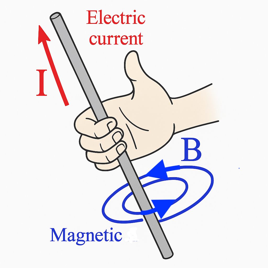
The right-hand rule showing the relationship between current (I) and the resulting magnetic field (B).
This right-hand rule is the foundation for understanding how current-carrying wires generate magnetic fields. It illustrates that magnetic field lines form concentric circles around a straight current-carrying wire, with the direction determined by the right hand.
Example: A straight wire carries a current flowing upward. Using the right-hand rule, determine the direction of the magnetic field at points to the east, west, north, and south of the wire.
Solution:
Using the right-hand rule with thumb pointing upward (direction of current):
- At a point east of the wire: The magnetic field points south (toward you)
- At a point west of the wire: The magnetic field points north (away from you)
- At a point north of the wire: The magnetic field points west (to the right)
- At a point south of the wire: The magnetic field points east (to the left)
This confirms that the magnetic field forms concentric circles around the wire in a counterclockwise direction when viewed from above (looking in the direction of the current).
Right-Hand Rule for Current, Velocity, and Magnetic Field
I-V-B Right-Hand Rule:
Point your right hand with your thumb, index finger, and middle finger mutually perpendicular to each other (forming three axes of a coordinate system):
- Thumb: Direction of the current (I) or motion of positive charges
- Index finger: Direction of the external magnetic field (B)
- Middle finger: Direction of the resulting force or voltage (V)
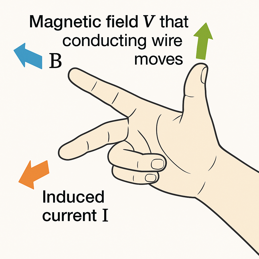
The I-V-B right-hand rule showing the relationship between current direction (I), magnetic field direction (B), and the resulting force or voltage (V).
This right-hand rule is useful for determining the direction of:
- The force on a current-carrying wire in a magnetic field
- The force on a moving charged particle in a magnetic field
- The induced voltage in a conductor moving through a magnetic field
Example: A horizontal wire carries a current flowing east and is placed in a vertical magnetic field pointing downward. Using the right-hand rule, determine the direction of the force on the wire.
Solution:
Using the I-V-B right-hand rule:
- Thumb (I): Points east (direction of current)
- Index finger (B): Points downward (direction of magnetic field)
- Middle finger (V/F): To maintain perpendicularity with both I and B, the middle finger points north (direction of force)
Therefore, the wire experiences a force in the northward direction. This can be verified using the formula \(\vec{F} = I \vec{l} \times \vec{B}\).
Understanding these right-hand rules is essential for solving problems involving electromagnetic interactions and for visualizing the three-dimensional relationships between electrical and magnetic quantities.
Charged Particle in a Magnetic Field
\(r = \frac{mv}{qB} \qquad f = \frac{q B}{2\pi m}\)
Where:
- \(r\) = radius of the circular path
- \(m\) = mass of the particle
- \(v\) = velocity of the particle
- \(q\) = charge of the particle
- \(B\) = magnetic field strength
- \(f\) = frequency of revolution
Simple Harmonic Motion Equations
\(x(t) = A \cos (\omega t + \phi_0)\)
\(v_x(t) = -\omega A \sin (\omega t + \phi_0) = -v_{\max} \sin (\omega t + \phi_0)\)
\(v_{\max} = \frac{2\pi A}{T} = 2\pi f A = \omega A\)
\(a_x(t) = -\omega^2 A \cos (\omega t + \phi_0) = -a_{\max} \cos (\omega t + \phi_0)\)
\(\omega = \sqrt{\frac{k}{m}} = \sqrt{\frac{g}{L}} \qquad f = \frac{\omega}{2\pi} \qquad T = \frac{1}{f}\)
\(E = K + U = \frac{1}{2}mv_x^2 + \frac{1}{2}k x^2 = \frac{1}{2} k A^2 = \frac{1}{2}m (v_{\max})^2\)
Where:
- \(x(t)\) = position as a function of time
- \(A\) = amplitude (maximum displacement from equilibrium)
- \(\omega\) = angular frequency (radians per second)
- \(t\) = time
- \(\phi_0\) = initial phase constant
- \(v_x(t)\) = velocity as a function of time
- \(v_{\max}\) = maximum velocity
- \(a_x(t)\) = acceleration as a function of time
- \(a_{\max}\) = maximum acceleration
- \(k\) = spring constant
- \(m\) = mass
- \(g\) = acceleration due to gravity
- \(L\) = length (for a pendulum)
- \(f\) = frequency (oscillations per second)
- \(T\) = period (time for one complete oscillation)
- \(E\) = total energy
- \(K\) = kinetic energy
- \(U\) = potential energy
Simple harmonic motion (SHM) is a type of periodic motion where the restoring force is directly proportional to the displacement and acts in the direction opposite to that of displacement. Examples include a mass on a spring and a simple pendulum (for small angles).
Example: A 0.2 kg mass attached to a spring with spring constant 8 N/m oscillates with an amplitude of 0.1 m. Calculate:
- The angular frequency
- The period and frequency
- The maximum velocity
- The total energy
Solution:
1. Angular frequency: \(\omega = \sqrt{\frac{k}{m}} = \sqrt{\frac{8 \text{ N/m}}{0.2 \text{ kg}}} = \sqrt{40} \approx 6.32 \text{ rad/s}\)
2. Period: \(T = \frac{2\pi}{\omega} = \frac{2\pi}{6.32} \approx 0.99 \text{ s}\)
Frequency: \(f = \frac{1}{T} = \frac{1}{0.99} \approx 1.01 \text{ Hz}\)
3. Maximum velocity: \(v_{\max} = \omega A = 6.32 \times 0.1 = 0.632 \text{ m/s}\)
4. Total energy: \(E = \frac{1}{2}kA^2 = \frac{1}{2} \times 8 \times (0.1)^2 = 0.04 \text{ J}\)
Wave Phenomena
\(I = \frac{P}{A}\)
\(v_{\text{string}} = \sqrt{\frac{T_s}{\mu}}\)
\(\beta = (10\ \mathrm{dB}) \log_{10} \left( \frac{I}{1 \times 10^{-12}} \right)\)
\(v = \lambda f \qquad \omega = 2\pi f = \frac{2\pi}{T} \qquad k = \frac{2\pi}{\lambda}\)
\(D(x,t) = A \sin (kx - \omega t + \phi_0)\)
\(\Delta \phi = 2\pi \frac{\Delta x}{\lambda} + \Delta \phi_0\)
Where:
- \(I\) = intensity (power per unit area)
- \(P\) = power
- \(A\) = area
- \(v_{\text{string}}\) = wave speed on a string
- \(T_s\) = tension in the string
- \(\mu\) = linear mass density (mass per unit length)
- \(\beta\) = sound intensity level in decibels
- \(v\) = wave speed
- \(\lambda\) = wavelength
- \(f\) = frequency
- \(\omega\) = angular frequency
- \(T\) = period
- \(k\) = wave number
- \(D(x,t)\) = displacement as a function of position and time
- \(A\) = amplitude
- \(\phi_0\) = initial phase
- \(\Delta \phi\) = phase difference
- \(\Delta x\) = path difference
Wave phenomena describe how disturbances propagate through a medium or space. This includes mechanical waves (like sound and water waves) and electromagnetic waves (like light).
Example 1: A string with a linear mass density of 0.01 kg/m is under a tension of 40 N. Calculate the speed of a wave on this string.
Solution:
Using the formula for wave speed on a string: \(v_{\text{string}} = \sqrt{\frac{T_s}{\mu}}\)
\(v_{\text{string}} = \sqrt{\frac{40 \text{ N}}{0.01 \text{ kg/m}}} = \sqrt{4000} \approx 63.2 \text{ m/s}\)
Example 2: A sound wave has a frequency of 440 Hz and a speed of 343 m/s. Calculate its wavelength and wave number.
Solution:
Wavelength: \(\lambda = \frac{v}{f} = \frac{343 \text{ m/s}}{440 \text{ Hz}} \approx 0.78 \text{ m}\)
Wave number: \(k = \frac{2\pi}{\lambda} = \frac{2\pi}{0.78} \approx 8.05 \text{ rad/m}\)
Doppler Effect
\(f_+ = f_0 \frac{v+v_0}{v} \qquad f_- = f_0 \frac{v-v_0}{v}\)
\(f_+ = (1+\frac{v_0}{v}) f_0 \qquad f_- = (1-\frac{v_0}{v}) f_0\)
\(f_{\text{observed}} = f_0 \frac{1+v_0/v}{1-v_s/v}\)
Where:
- \(f_+\) = observed frequency when source and observer move toward each other
- \(f_-\) = observed frequency when source and observer move away from each other
- \(f_0\) = source frequency (emitted frequency)
- \(v\) = wave speed in the medium
- \(v_0\) = observer velocity relative to the medium (positive when moving toward the source)
- \(v_s\) = source velocity relative to the medium (positive when moving toward the observer)
- \(f_{\text{observed}}\) = frequency observed in the general case
The Doppler effect is the change in frequency of a wave in relation to an observer moving relative to the wave source. It occurs for all types of waves, including sound waves and electromagnetic waves like light.
Example: A police car with a siren emitting a sound at 500 Hz is moving at 25 m/s toward a stationary observer. The speed of sound in air is 343 m/s. Calculate the frequency heard by the observer.
Solution:
In this case, the observer is stationary (\(v_0 = 0\)) and the source is moving toward the observer at \(v_s = 25 \text{ m/s}\).
Using the general Doppler formula: \(f_{\text{observed}} = f_0 \frac{1+v_0/v}{1-v_s/v}\)
\(f_{\text{observed}} = 500 \text{ Hz} \times \frac{1+0}{1-25/343} = 500 \text{ Hz} \times \frac{1}{1-0.073} = 500 \text{ Hz} \times \frac{1}{0.927} \approx 539 \text{ Hz}\)
The observer hears a higher frequency (539 Hz) than the emitted frequency (500 Hz), which is the characteristic of the Doppler effect when a source approaches an observer.
Standing Waves
\(D(x, t) = A(x) \cos \omega t\)
\(A(x) = 2a \sin kx\)
\(\lambda_m = \frac{2L}{m} \qquad m=1,2,3,4\dots\)
\(D_m = [2a \cos (\Delta \phi / 2)] \sin (k x_{\text{avg}} - \omega t + (\phi_0)_{\text{avg}})\)
\(f_m = \frac{v}{\lambda_m} = \frac{v m}{2L},\quad m=1,2,3,4\dots\)
\(\lambda_m = \frac{4L}{m},~m=1,3,5,7\dots\)
\(f_m = \frac{m v}{4L} = m f_1\)
Where:
- \(D(x,t)\) = displacement of the standing wave as a function of position and time
- \(A(x)\) = amplitude as a function of position
- \(a\) = maximum amplitude of the constituent traveling waves
- \(\omega\) = angular frequency
- \(t\) = time
- \(k\) = wave number
- \(x\) = position along the wave
- \(\lambda_m\) = wavelength of the mth harmonic (mode)
- \(L\) = length of the medium (string, pipe, etc.)
- \(m\) = mode number (integer)
- \(D_m\) = displacement for mode m
- \(\Delta \phi\) = phase difference
- \(x_{\text{avg}}\) = average position
- \((\phi_0)_{\text{avg}}\) = average initial phase
- \(f_m\) = frequency of the mth harmonic
- \(v\) = wave speed
- \(f_1\) = fundamental frequency (first harmonic)
Standing waves are formed when two waves of the same frequency traveling in opposite directions interfere with each other. They appear to stand still, with fixed positions of zero displacement (nodes) and maximum displacement (antinodes). Standing waves are fundamental in understanding musical instruments, resonance, and quantum mechanics.
Example: A guitar string is 65 cm long and fixed at both ends. The wave speed on the string is 240 m/s.
- Calculate the frequencies of the first three harmonics (modes).
- What are the wavelengths of these harmonics?
Solution:
For a string fixed at both ends, we use the formula: \(f_m = \frac{v m}{2L}\) and \(\lambda_m = \frac{2L}{m}\)
With \(L = 0.65 \text{ m}\) and \(v = 240 \text{ m/s}\):
1. First harmonic (m = 1):
\(f_1 = \frac{240 \times 1}{2 \times 0.65} = \frac{240}{1.3} \approx 184.6 \text{ Hz}\)
\(\lambda_1 = \frac{2 \times 0.65}{1} = 1.3 \text{ m}\)
2. Second harmonic (m = 2):
\(f_2 = \frac{240 \times 2}{2 \times 0.65} = \frac{480}{1.3} \approx 369.2 \text{ Hz}\)
\(\lambda_2 = \frac{2 \times 0.65}{2} = 0.65 \text{ m}\)
3. Third harmonic (m = 3):
\(f_3 = \frac{240 \times 3}{2 \times 0.65} = \frac{720}{1.3} \approx 553.8 \text{ Hz}\)
\(\lambda_3 = \frac{2 \times 0.65}{3} \approx 0.433 \text{ m}\)
Diffraction and Interference
\(\theta_m = m \frac{\lambda}{d}\)
\(y_m = m \frac{\lambda L}{d}\)
\(\theta'_m = \left(m+\frac{1}{2}\right) \frac{\lambda}{d}\)
\(y'_m = \left(m+\frac{1}{2}\right) \frac{\lambda L}{d}\)
\(d \sin \theta_m = m\lambda,~y_m = L \tan \theta_m, \quad m = 0,1,2,3,4\)
\(a \sin \theta_m = m\lambda,\quad m=1,2,3,4\)
\(\sin\theta_1 = 1.22 \frac{\lambda}{D}\)
Where:
- \(\theta_m\) = angle to the mth constructive interference maximum (bright fringe)
- \(\theta'_m\) = angle to the mth destructive interference minimum (dark fringe)
- \(m\) = order of maximum/minimum (integer)
- \(\lambda\) = wavelength of light
- \(d\) = separation between slits or sources
- \(y_m\) = linear distance from central maximum to mth bright fringe on a screen
- \(y'_m\) = linear distance from central maximum to mth dark fringe on a screen
- \(L\) = distance from slits to screen
- \(a\) = width of a single slit
- \(D\) = diameter of circular aperture
Diffraction is the bending of waves around obstacles or through openings, while interference is the superposition of waves resulting in a new wave pattern. These phenomena are key to understanding the wave nature of light and other waves.
Example 1 (Double-slit interference): Light with a wavelength of 550 nm passes through two slits separated by 0.1 mm. The interference pattern is observed on a screen 2 m away. Calculate the positions of the first three bright fringes (maxima) from the central maximum.
Solution:
Using the formula \(y_m = m \frac{\lambda L}{d}\) where:
\(\lambda = 550 \times 10^{-9} \text{ m}\)
\(L = 2 \text{ m}\)
\(d = 0.1 \times 10^{-3} \text{ m}\)
First maximum (m = 1): \(y_1 = 1 \times \frac{550 \times 10^{-9} \times 2}{0.1 \times 10^{-3}} = 0.011 \text{ m} = 11 \text{ mm}\)
Second maximum (m = 2): \(y_2 = 2 \times \frac{550 \times 10^{-9} \times 2}{0.1 \times 10^{-3}} = 0.022 \text{ m} = 22 \text{ mm}\)
Third maximum (m = 3): \(y_3 = 3 \times \frac{550 \times 10^{-9} \times 2}{0.1 \times 10^{-3}} = 0.033 \text{ m} = 33 \text{ mm}\)
Example 2 (Single-slit diffraction): Light with a wavelength of 650 nm passes through a single slit of width 0.05 mm. Calculate the angle to the first minimum in the diffraction pattern.
Solution:
For a single slit, the minima occur at angles given by \(a \sin \theta_m = m\lambda\) for \(m = 1, 2, 3, ...\)
For the first minimum (m = 1):
\(\sin \theta_1 = \frac{1 \times 650 \times 10^{-9}}{0.05 \times 10^{-3}} = 0.013\)
\(\theta_1 = \sin^{-1}(0.013) \approx 0.75°\)
Optics
\(n_1 \sin \theta_1 = n_2 \sin \theta_2\)
\(\theta_c = \sin^{-1} \left( \frac{n_2}{n_1} \right)\)
\(n = \frac{c}{v}\)
Where:
- \(n_1\) = refractive index of medium 1
- \(n_2\) = refractive index of medium 2
- \(\theta_1\) = angle of incidence
- \(\theta_2\) = angle of refraction
- \(\theta_c\) = critical angle for total internal reflection
- \(n\) = refractive index of a medium
- \(c\) = speed of light in vacuum
- \(v\) = speed of light in the medium
Optics is the branch of physics that studies the behavior of light, including its interactions with matter and the construction of instruments that use or detect it. The formulas above describe refraction (Snell's Law), total internal reflection, and the definition of refractive index.
Example 1 (Refraction): Light travels from air (n₁ = 1.00) into water (n₂ = 1.33). If the angle of incidence is 45°, what is the angle of refraction?
Solution:
Using Snell's Law: \(n_1 \sin \theta_1 = n_2 \sin \theta_2\)
\(1.00 \times \sin 45° = 1.33 \times \sin \theta_2\)
\(\sin \theta_2 = \frac{1.00 \times \sin 45°}{1.33} = \frac{0.7071}{1.33} \approx 0.5317\)
\(\theta_2 = \sin^{-1}(0.5317) \approx 32.1°\)
Example 2 (Total Internal Reflection): Calculate the critical angle for light traveling from water (n₁ = 1.33) to air (n₂ = 1.00).
Solution:
Using the formula for critical angle: \(\theta_c = \sin^{-1} \left( \frac{n_2}{n_1} \right)\)
\(\theta_c = \sin^{-1} \left( \frac{1.00}{1.33} \right) = \sin^{-1}(0.7519) \approx 48.6°\)
This means that if light hits the water-air boundary at an angle greater than 48.6° from the normal, total internal reflection will occur.
Nuclear Physics
\(B = \left[Z m_{^1\mathrm{H}} + N m_n - m_{\text{atom}}\right] \times (931.494~\mathrm{MeV/u})\)
\(A = A_0 e^{-\lambda t} = A_0 e^{- t / \tau}\)
\(N = N_0 e^{-\lambda t} = N_0 e^{- t / \tau} = N_0 \left( \frac{1}{2} \right)^{t/t_{1/2}}\)
\(t_{1/2} = \frac{\ln 2}{\lambda},\quad \tau = \frac{1}{\lambda}\)
\(R = r_0 A^{1/3}\)
Where:
- \(B\) = binding energy of the nucleus
- \(Z\) = atomic number (number of protons)
- \(N\) = number of neutrons
- \(m_{^1\mathrm{H}}\) = mass of a hydrogen atom
- \(m_n\) = mass of a neutron
- \(m_{\text{atom}}\) = actual mass of the atom
- \(A\) = activity (number of decays per second)
- \(A_0\) = initial activity
- \(\lambda\) = decay constant
- \(t\) = time
- \(\tau\) = mean lifetime
- \(N\) = number of undecayed nuclei
- \(N_0\) = initial number of nuclei
- \(t_{1/2}\) = half-life (time for half the nuclei to decay)
- \(R\) = nuclear radius
- \(r_0\) = constant (approximately 1.2 × 10⁻¹⁵ m)
- \(A\) = mass number (number of nucleons = Z + N)
Nuclear physics studies the components, structure, and behavior of atomic nuclei. The formulas above relate to nuclear binding energy, radioactive decay, and nuclear size.
Example 1 (Radioactive Decay): A radioactive sample has an initial activity of 800 Bq and a half-life of 5 hours. Calculate:
- The decay constant
- The activity after 15 hours
Solution:
1. Decay constant: \(\lambda = \frac{\ln 2}{t_{1/2}} = \frac{\ln 2}{5 \text{ h}} = \frac{0.693}{5} \approx 0.1386 \text{ h}^{-1}\)
2. Activity after 15 hours: \(A = A_0 e^{-\lambda t} = 800 \text{ Bq} \times e^{-0.1386 \times 15} = 800 \text{ Bq} \times e^{-2.079} = 800 \text{ Bq} \times 0.125 = 100 \text{ Bq}\)
Alternatively, we can use the half-life formula: \(A = A_0 \left( \frac{1}{2} \right)^{t/t_{1/2}} = 800 \text{ Bq} \times \left( \frac{1}{2} \right)^{15/5} = 800 \text{ Bq} \times \left( \frac{1}{2} \right)^3 = 800 \text{ Bq} \times \frac{1}{8} = 100 \text{ Bq}\)
Example 2 (Nuclear Radius): Calculate the radius of a uranium-238 nucleus (A = 238).
Solution:
Using the formula: \(R = r_0 A^{1/3}\) with \(r_0 = 1.2 \times 10^{-15} \text{ m}\) and \(A = 238\):
\(R = 1.2 \times 10^{-15} \times 238^{1/3} = 1.2 \times 10^{-15} \times 6.18 = 7.42 \times 10^{-15} \text{ m} = 7.42 \text{ fm}\)
Applications of Magnetism
Magnetism has numerous practical applications in our daily lives and in technology:
- Electric motors and generators
- Magnetic resonance imaging (MRI) in medicine
- Magnetic storage devices (hard drives)
- Electromagnetic induction for power generation
- Magnetic levitation for transportation
- Particle accelerators in research
Example: Calculate the magnetic field 5 cm from a wire carrying a current of 2 A.
Using \(B = \frac{\mu_0 I}{2\pi d}\):
\(B = \frac{4\pi \times 10^{-7} \times 2}{2\pi \times 0.05} = \frac{8\pi \times 10^{-7}}{2\pi \times 0.05} = \frac{4 \times 10^{-7}}{0.05} = 8 \times 10^{-6}\) T